
GRIN Material Property in QUADOA® Optical CAD
The GRIN material property in QUADOA® Optical CAD assigns a gradient-index profile to any lens material. It is used to simulate classical GRIN lenses, to tolerance refractive index inhomogeneities, and to model thermal lensing in high-power laser systems. Rays follow curved paths through the medium, calculated with a Runge-Kutta method, and the GRIN parameters can be optimized like any other parameter.
Key points
- Applications: GRIN lenses, index inhomogeneity tolerancing and thermal lensing.
- Profiles: radial, axial, spherical, Luneburg, Rochester, 2D grid and 3D grid.
- A profile can describe a refractive index or a temperature distribution, relative or absolute.
- Assign a profile with a right-click on the material icon or in the Construction tab.
- GRIN parameters can be optimized with the variable icon.
- The Z Step sets the accuracy of the Runge-Kutta ray integration.
- Only one GRIN profile per material is used.
- The GRIN axis is defined in the element coordinate system, and GRIN works with any surface type.
Terms used in this article
- GRIN (gradient index)
- A material whose refractive index varies with position inside the element.
- Eikonal equation
- The equation that describes the ray path in a medium with varying refractive index.
- Runge-Kutta method
- An iterative numerical method used to solve the eikonal equation step by step.
- Z Step
- The step size of the Runge-Kutta iteration, common to all GRIN profiles.
How to assign a GRIN profile to a lens
- In the Optical Design Editor, expand the lens, for example a singlet.
- Right-click the material icon and choose a GRIN profile from the drop-down menu. Alternatively, choose the profile on the far right of the Construction tab.
- Select, for example, the radial GRIN profile.
- Enter the profile coefficients, for example from your GRIN material manufacturer.
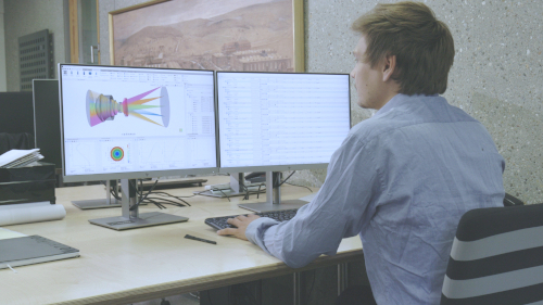
The 3D view now shows the curved ray paths inside the GRIN medium. The system can be analyzed with all plots in the Analysis tab, and the GRIN parameters can be optimized by activating their variable icon.
Which GRIN profiles are available?
All profiles are defined in the local coordinate system of the element (x, y, z). Polynomial profiles have a Polynomial Order and coefficients A1, A2, …
| Profile | Definition | Typical use |
|---|---|---|
| Radial | Δn = A1·r + A2·r² + A3·r³ + …, with r = √(x² + y²) | Classical radial GRIN lenses |
| Axial | Polynomial in y or x (parameter Axis) | Index gradient in one lateral direction |
| Spherical | Polynomial in the distance from a center Z0 on the element axis | Spherically symmetric gradients |
| Luneburg | n = n0·√(2 − r²/A²), with r measured from a center at z = Radius | Lüneburg lenses |
| Rochester | Δn = NZz + NZ2z² + NZ3z³ + NZ4z⁴ + NR2r² + NR4r⁴ + NR6r⁶ + NR8r⁸ | GRIN materials described by the University of Rochester equation |
| 2D Grid | Arbitrary profile from a 2D interpolation table | Material inhomogeneities, thermal lensing from STOP analysis |
| 3D Grid | Arbitrary profile from a 3D interpolation table | Material inhomogeneities, thermal lensing from STOP analysis |
Index profile or temperature profile?
The Profile Type parameter defines what the profile describes and how it is applied:
| Profile Type | Resulting refractive index |
|---|---|
| Relative Index | n = n(λ, T) + nProfile(x, y, z): the profile is added to the base index of the material |
| Absolute Index | n = nProfile(x, y, z): the base index of the material is ignored |
| Relative Temperature | n = n(λ, T + TProfile(x, y, z)): the profile is a temperature change added to the material temperature |
| Absolute Temperature | n = n(λ, TProfile(x, y, z)): the profile is the absolute temperature |
The temperature types are useful for thermal lensing: a temperature field, for example from a thermal simulation of a laser optic, is converted into an index distribution using the thermal data of the glass. Only one GRIN profile per material is evaluated; if several are defined, only the first one is used.
How to choose the step size (Z Step)
The ray path through a GRIN medium is found by solving the eikonal equation with an iterative algorithm based on the Runge-Kutta method. The step size of each iteration is set with the Z Step parameter, which is common to all GRIN profiles.
- A smaller step increases the accuracy but also the computation time.
- Recommended approach: start with a large value, for example 5, and reduce it step by step until the results change by less than an acceptable tolerance.
Why is the GRIN axis defined in the element coordinate system?
The GRIN profile is defined in the local coordinate system of the lens, not in the coordinate system of a surface. Its axis is therefore independent of the surfaces, which is essential for realistic tolerancing. The video compares three configurations:
| Configuration | First surface | Element and GRIN axis |
|---|---|---|
| 1 | Not tilted | Not tilted |
| 2 | Tilted | Not tilted |
| 3 | Tilted | Tilted |
The refraction at the tilted first surface is identical in configurations 2 and 3, but the ray paths inside the medium differ, because the GRIN axis is tilted only in configuration 3. A surface tilt tolerance therefore does not tilt the GRIN profile, just as in a real lens.
Can GRIN be combined with aspheres and freeforms?
Yes. The surfaces of a GRIN lens are not limited to a specific shape or phase type. You can use GRIN profiles with any surface or form type in the Construction tab, including freeform lenses and diffractive optics. This is important, for example, to simulate the index inhomogeneity of an aspheric lens. For index inhomogeneities in tolerance or STOP analysis, see also the Building optical systems articles in the Learning Center.
Video tutorial: the GRIN material property
This 5-minute video shows how to assign a GRIN profile, set the step size and why the GRIN axis is defined in the element coordinate system.
Video length: 4:53 min · Also on YouTube: GRIN Material Property in QUADOA® Optical CAD
Frequently asked questions
To simulate classical gradient-index lenses, to tolerance refractive index inhomogeneities, and to model thermal lensing in high-power laser systems.
Radial, axial, spherical, Luneburg, Rochester, 2D grid and 3D grid GRIN profiles.
Yes. With the Profile Type Relative Temperature or Absolute Temperature, the profile defines a temperature field, from which the refractive index is calculated. This is used, for example, to model thermal lensing.
The ray path is calculated with a Runge-Kutta method. The Z Step parameter sets the step size: smaller steps are more accurate but slower. Start with a large value, for example 5, and reduce it until the results stop changing significantly.
No. The GRIN profile is defined in the element coordinate system, so tilting a single surface does not tilt it. Tilting the whole element does.
Yes. GRIN profiles work with any surface or form type, including aspheres, freeforms and diffractive surfaces.
Yes. Like all parameters in the Optical Design Editor, GRIN parameters become optimization variables when you activate their variable icon.